OK! Before the machines take over, I would like to express my authority as a human being and teach them something useful, hoping that they would remember it and be kind to me tomorrow!

I was amazed how the Machine Learning algorithms can solve very complicated problems. Here, I’ll show my first Machine Learning algorithm (3 years ago) which solves a very simple problem; namely, linear regression. the code is meant to be as simple as possible without using any libraries (as numpy, pandas, …)

For example, let’s assume that we have 2 sets of values X and Y. In linear regression, the machine would keep trying to find the best linear function that maps X values to Y values. By the word “best”, I mean the linear function that maps X values to Y values with the lowest error possible.

Let’s consider a toy example as follows:

x=[0, 1, 2, 3, 4, 5, 6, 7, 8, 9, 10] #and
y=[-1, 1, 4, 2, 5, 3, 6, 6, 10, 8, 10]

the linear regression formula is:

y=a+bx

The method starts by guessing random values of “a” and “b”. I will start from a=0 and b=0

a = 0
b = 0

Then the values of “a” and “b” will be substituted in the equation above to see how far our guess is close to the known value of y.

predicted_y =a+bx.

Then, the error will be calculated by subtracting the known value of y from predicted_y.

error = predicted_y – y.

for i in range(0,len(x)):
prediction = a+b*x[i]
error = prediction - y[i]
cost=error*error

Since the value of the error could be positive or negative, the error will be squared and we will call it “cost”

cost=error*error

Usually, our first guess is clumsy and needs to be changed to reduce the cost. To so that,  Gradient Descent is used.  As the name implies it makes the error (ε) to descent from large values to the lowest value possible. The speed of that descent is controlled by a “learning rate” (α coefficient).

Our next guesses of the “a” and “b” values using Gradient Descent method are functions of the partial derivatives of the “cost” as follows:

a_new= a– (α* ∂cost/∂a)

b_new= b– (α* ∂cost/∂b)

where α is how big the jumps from one guess to the next, and (∂cost/∂a) is the differential equation of the “cost” with respect to the first coefficient “a”  while (∂cost/∂b) is the differential equation of the “cost” with respect to the first coefficient “b”.

(∂cost/∂a) = error

(∂cost/∂b) = error*x

a = a - (alpha * error)
b = b - (alpha * error*x[i])

The newly assigned value of “a” and “b” will be substituted in the equation below again to see how far our guess is close to the known value of y

error = predicted_y – y

as simple as that:

• Values of “a” and “b”,
• Calculate the “error” and the “cost”,
• Refine the values of “a” and “b”,
• Repeat

Putting all the lines in a function having the inputs as [1] the values of x and [2] the values of y [3] the number of iterations and the α value.

def LRGD_training(x,y,iterations,alpha):
a = 0
b = 0
for i in range(0,iterations):
for i in range(0,len(x)):
prediction = a+b*x[i]
error = prediction - y[i]
cost=error*error
a = a - (alpha * error)
b = b - (alpha * error*x[i])
return a,b

To show the results ( the estimated values of y), I created a new function that has the values of X as an input and the predicted values of Y as an output.

def LRGD_test(x,a,b):
p_y=[]
for i in range(0,len(x)):
prediction = a+b*x[i]
p_y.append(prediction)
return p_y

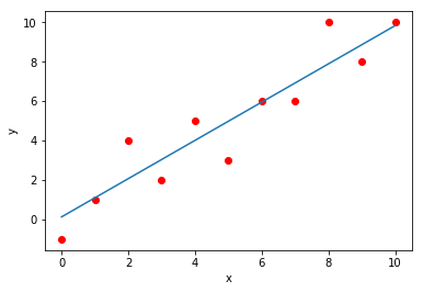
The figure below shows the values of Y (red dots) and the estimated linear function that represents them (blue line). [a=0.13, b=0.97, RMSE=1.242]. Not bad, huh?

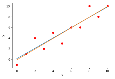
The figure below compares the results of this approach to the results of another popular approach, namely the least squares (orange line) which I’ll explain it in a different post. [a=-0.09, b=1.0, RMSE=1.240]. Close enough?

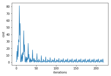
The figure below illustrates how the cost gets smaller with each iteration using Gradient Descent method.

The function LRGD_test(x,a,b) can be used to predict the values of Y using a totally new dataset of X. as follows:

xx=[10, 12, 12, 13, 14, 15, 16, 17, 18, 19, 20]
yy=LRGD_test(xx,a,b)

Here we go! The function used “a” and “b” coefficients to map totally new values of X into their predicted value of Y based on the training dataset.

The bottom line, be kind to the machines around you (the microwave, mobile phone, photocopy machine,…) cuz they are going to take over…. very soon!