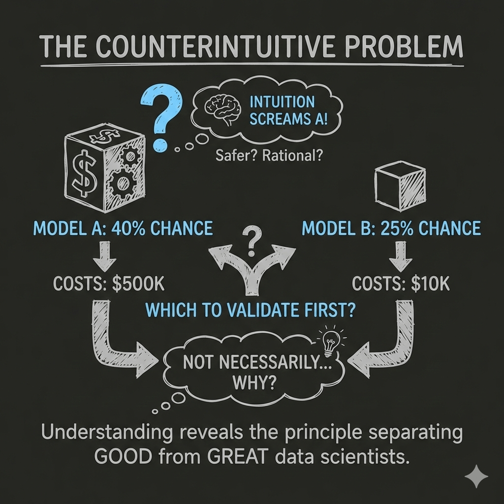
The Counterintuitive Problem

When leading my data science team, I usually find myself in a situation where I need to evaluate two potential ML models for production:

• Model A: 40% chance of meeting performance targets, but requires $500K in compute and engineering to test and validate
• Model B: 25% chance of success, but only $10K to test and validate

Which would you validate first?

If you’re like most people, your intuition screams “Model A!” It is higher in probability, so it feels safer. It’s the rational choice, right?

Not necessarily.. and understanding why reveals a fundamental principle that separates good data scientists from great ones.

---

Understanding the Baseline: What Does Success Look Like?

Before we dive into the strategies, let’s establish what “success” means in this scenario.

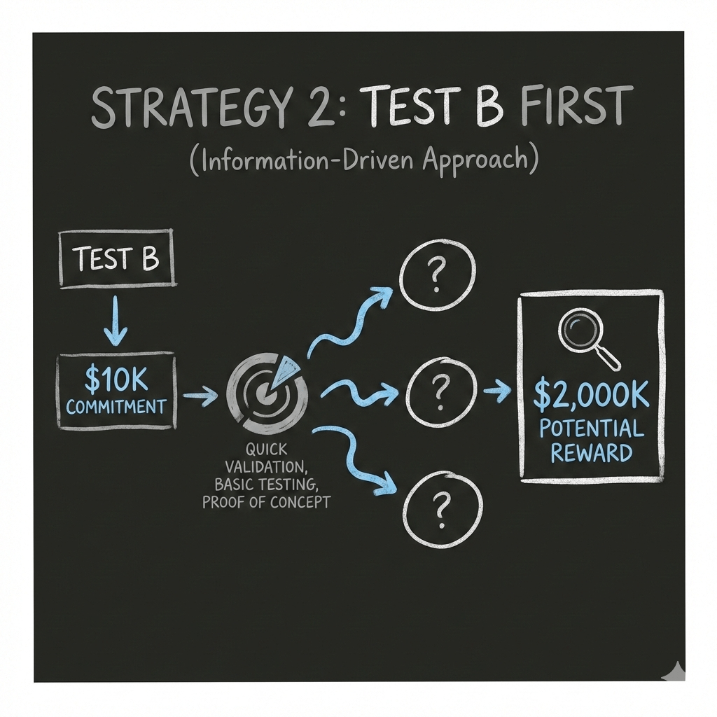
The Reward: If either model meets your performance targets, it generates $2,000K in value to your company. This reward could be:

• Annual revenue increase from better recommendations
• Cost savings from more efficient operations
• Competitive advantage worth this much to stakeholders

The Question: Looking back at the options above, should you spend $500K to test the 40% probability option, or $10K to test the 25% probability option first?

I emphasised the word first, as the order in which you test these models determines not just your expected profit, but your risk exposure, capital efficiency, and learning trajectory.

---

Strategy 1: Test A First (The Intuitive Approach)

Let’s see this decision and the consequences would be (I’ll explain every calculation, don’t worry).

STEP 1: You commit $500K to Test Model A

The moment you start testing Model A, you’ve committed $500K. This money is gone regardless of the outcome. Let’s say it pays for:

• GPU compute time for training
• Engineering hours for implementation
• Data pipeline development
• Validation infrastructure

Critical Point: This $500K is a sunk cost the moment you begin. You cannot get it back.

Now we wait for the results. There are three possible scenarios:

SCENARIO 1: Model A Succeeds (40% probability of success)

What would happen:

• Your $500K investment pays off
• Model A meets performance targets
• You deploy it and capture the $2,000K in value
• You stop testing (no need to try Model B)

Financial Accounting:

Revenue from deploying Model A:    +$2,000K
Money spent testing A:             -$500K
───────────────────────────────────────────
Net Profit:                        +$1,500K

Why $1,500K and not $2,000K?
Because you had to spend $500K to discover that Model A works. That’s the cost of validation. Your gross revenue is $2,000K, but your net profit (revenue minus costs) is $1,500K

Expected contribution: remember this model has a 40% probability of success. This means that this happens 40% of the time, also meaning in a mathematical form:

0.40 × $1,500K = $600K

---

SCENARIO 2: Model A Fails, Then B Succeeds

Let’s say we test Model A for $500K and it fails to validate, then

• You’re down $500K with nothing to show for it
• But you don’t give up! You still have Model B
• You spend another $10K to test Model B
• Model B succeeds and captures the $2,000K value

Financial Accounting:

Money already spent on A:           -$500K (sunk cost)
Revenue from A:                      $0 (it failed)
Additional cost to test B:          -$10K
Revenue from deploying B:           +$2,000K
─────────────────────────────────────────────
Net Profit:                         +$1,490K

Probability Calculation:
This scenario requires TWO things to happen:

1. Model A must fail: 60% chance (100% – 40% = 60%)
2. Model B must succeed: 25% chance

Combined probability = 0.60 × 0.25 = 0.15 or 15%

Why multiply? Because both events must occur in sequence.

Note: we assumed that the two solutions are independent (the failure of one solution does not tell you anything about the other); yet this is not always the case. We will talk about this later in the post.

Expected contribution to total Expected Value: 0.15 × $1,490K = $223.5K

---

SCENARIO 3: Both Models Fail

If Model A fails (after spending $500K) and Model B also fails (after spending $10K more)

• You’ve exhausted all options
• No revenue is generated

Financial Accounting:

Money spent testing A:              -$500K
Revenue from A:                     $0 (failed)
Money spent testing B:              -$10K
Revenue from B:                     $0 (failed)
─────────────────────────────────────────────
Total Loss:                         -$510K

Probability Calculation:
This requires TWO failures:

1. Model A fails: 60% chance
2. Model B also fails: 75% chance (100% – 25% = 75%)

Combined probability = 0.60 × 0.75 = 0.45 or 45%

Important Insight: This is the most likely outcome! Almost half the time, you’ll lose $510K.

Expected contribution to total Expected Value: 0.45 × (-$510K) = -$229.5K

---

Calculating Expected Value for Strategy A→B

Expected Value is the probability-weighted average of all possible outcomes.

The Formula:

EV = (Prob of Outcome 1 × Value of Outcome 1)
   + (Prob of Outcome 2 × Value of Outcome 2)  
   + (Prob of Outcome 3 × Value of Outcome 3)

Plugging in our numbers:

EV(A→B) = (0.40 × $1,500K) + (0.15 × $1,490K) + (0.45 × -$510K)
        = $600K + $223.5K - $229.5K
        = $594K

What does this mean?
If you run this experiment 1,000 times, you’d average $594K profit per attempt. Some attempts you’d make $1,500K, some you’d lose $510K, but the average would be $594K.

---

Strategy 2: Test B First (The Information-Driven Approach)

Now let’s analyse testing Model B first. Same reward ($2,000K), same probabilities, but different cost structure.

STEP 1: You Commit $10K to Test Model B

Much smaller upfront investment, only $10K for:

• Quick prototype validation
• Basic performance testing
• Initial proof of concept

The Three Possible Outcomes

SCENARIO 1: Model B Succeeds (25% probability of success)

• Your $10K investment pays off immediately
• Model B meets performance targets
• You deploy it and capture the $2,000K value
• You stop testing (no need to try Model A)

Financial Accounting:

Revenue from deploying Model B:    +$2,000K
Money spent testing B:              -$10K
─────────────────────────────────────────────
Net Profit:                         +$1,990K

Why $1,990K is HUGE: You only spent $10K to unlock $2,000K in value. Compare this to Strategy A→B where early success gave you only $1,500K (because you spent $500K).

When the cheap test succeeds, you keep almost all the reward!

Probability: This happens 25% of the time. That means the expected contribution to total Expected Value= 0.25 × $1,990K = $497.5K

Compare to A→B: Testing A first contributed $600K from early success. Testing B first contributes only $497.5K from early success. So far, A→B seems better, right? Keep reading…

---

SCENARIO 2: Model B Fails, Then A Succeeds

• You test Model B for $10K .. it fails
• You’re down $10K but that’s manageable
• You still have Model A to try
• You spend $500K to test Model A
• Model A succeeds and captures the $2,000K value

Financial Accounting:

Money already spent on B:           -$10K (sunk cost)
Revenue from B:                     $0 (it failed)
Additional cost to test A:          -$500K
Revenue from deploying A:           +$2,000K
─────────────────────────────────────────────
Net Profit:                         +$1,490K

This is the SAME net profit as Strategy A→B’s Scenario 2! When the second test succeeds, you end up with $1,490K regardless of which order you tested.

Probability Calculation:

1. Model B must fail: 75% chance (100% - 25% = 75%)
2. Model A must succeed: 40% chance

Combined probability = 0.75 × 0.40 = 0.30 or 30%

HUGE DIFFERENCE: This scenario happens 30% of the time with B→A but only 15% of the time with A→B!

Why? Because B fails more often (75% vs 60%), which means you get more opportunities to try A as your second option.

Expected contribution to total EV: 0.30 × $1,490K = $447K

Compare to A→B: Testing A first, this scenario contributed $223.5K. Testing B first, it contributes $447K. That’s a $223.5K difference!

---

SCENARIO 3: Both Models Fail

• Model B fails (after spending $10K)
• Model A also fails (after spending $500K more)
• You’ve exhausted all options
• No revenue is generated

Financial Accounting:

Money spent testing B:              -$10K
Revenue from B:                     $0 (failed)
Money spent testing A:              -$500K
Revenue from A:                     $0 (failed)
─────────────────────────────────────────────
Total Loss:                         -$510K

Key Point: This is EXACTLY the same as Strategy A→B! Both fail, you lose $510K regardless of order.

Probability Calculation:

1. Model B fails: 75% chance
2. Model A also fails: 60% chance

Combined probability = 0.75 × 0.60 = 0.45 or 45%

Same probability as A→B: This outcome happens 45% of the time either way.

Expected contribution to total EV: 0.45 × (-$510K) = -$229.5K

---

Calculating Expected Value for Strategy B→A

EV(B→A) = (0.25 × $1,990K) + (0.30 × $1,490K) + (0.45 × -$510K)
        = $497.5K + $447K - $229.5K
        = $715K

---

The Comparison: Why B→A Wins by $121K

Let’s put the strategies side by side:

Strategy	Expected Value	Difference
Test A First (A→B)	$594K	—
Test B First (B→A)	$715K	+$121K

Testing B first gives you 20% more expected value! – Byt WHY?

Breaking Down Where the Advantage Comes From

Let’s look at each outcome’s contribution:

Outcome	A→B Contribution	B→A Contribution	Difference
First test succeeds	$600K (40% × $1,500K)	$497.5K (25% × $1,990K)	-$102.5K ❌
Second test succeeds	$223.5K (15% × $1,490K)	$447K (30% × $1,490K)	+$223.5K ✅
Both fail	-$229.5K (45% × -$510K)	-$229.5K (45% × -$510K)	$0 —
TOTAL	$594K	$715K	+$121K ✅

The Key Insight

Testing A first:

• ✅ Better if first test succeeds (+$102.5K advantage)
• ❌ Worse if first test fails (-$223.5K disadvantage)
• The disadvantage is LARGER than the advantage

Testing B first:

• ✅ You lose $102.5K when the first test succeeds (25% chance)
• ✅ You gain $223.5K when the first test fails (75% chance)
• The gain is more frequent and larger!

---

Why This Is Counterintuitive: The Psychology of Probability

Most people choose A→B because:

1. Probability bias: “40% is better than 25%”.. true, but it ignores costs
2. Loss aversion: Afraid to “waste” the first attempt on the lower probability
3. Sunk cost fallacy: Once $500K is spent, you’re pot-committed
4. Outcome focus: Thinking about “which will work” rather than “how do I learn efficiently”

But the math shows: information efficiency beats probability when costs differ dramatically.

---

The Core Principle: Information Gain Per Dollar

This isn’t about probability alone.. it’s about information efficiency. We can quantify this:

Information Gain per Dollar = Probability / Cost

Model A: 0.40 / $500K = 0.0008 per $1K
Model B: 0.25 / $10K = 0.0250 per $1K

Model B gives you 31x more information per dollar spent.

---

What if the models/solutions are dependent?

In the previous sections, we assumed that the two solutions are independent (the failure of one solution does not tell you anything about the other); yet this is not always the case in real life.

More on this topic in the next post (stay tuned)

---

When to Test the High-Probability Option First

The cheap-first heuristic isn’t universal. There are specific, mathematically provable conditions where testing the expensive, high-probability option first is actually optimal. Let’s explore each case with detailed examples and proofs.

More on this topic in the next post (stay tuned)