The word “bank” is ambiguous. It could mean a financial institution or the edge of a river. Humans resolve this instantly from context. Self-Attention is how transformers do the same thing and we’re going to watch it happen, number by number.

transformer : A neural network that reads all words in a sentence simultaneously and figures out how each word relates to every other word, rather than reading left to right one word at a time.

We’ll use a tiny sentence with 4 words, each given a 2-dimensional embedding (x, y). Small enough to calculate by hand. Rich enough to see everything.

embedding :A way of turning a word into a list of numbers so a computer can do math on it — words with similar meanings end up with similar numbers.

Our Vocabulary:

we will study this sentence: “walk near river bank”

it consists of 4 words, and let’s assume that their embeddings are the following

• walk – its embeddings (x=0.1, y=0.9)
• near – its embeddings (x=0.5, y=0.5)
• river – its embeddings (x=0.8, y=0.8)
• bank – its embeddings (x=0.8, y=0.5)

The word “bank” is highlighted because it’s our protagonist, as it is the ambiguous word whose meaning the attention mechanism will help resolve. Is it the bank (where the money lives) or is it the bank (river side)?
You might be wondering, “Isn’t it obvious from the context? The word river is just next to it!” – well, it is easy for you, human, but not for the machine.

Moreover, the embedding of the word “bank” is fixed (x=0.8, y=0.5) .. If the embedding reflects the meaning, how does it behave when it has two meanings?

Our input matrix E (4 words × 2 dimensions):

E = [[0.1, 0.9],   ← walk
     [0.5, 0.5],   ← near
     [0.8, 0.8],   ← river
     [0.8, 0.5]]   ← bank

When the word “bank” is trying to understand its own meaning in context, it asks a question. Think of it like “bank” broadcasting:

“Hey everyone — I’m ambiguous. I could mean money or water. What’s around me that helps me figure out who I am?”

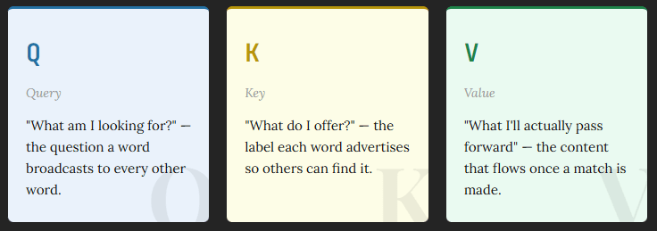
this question is called the Query.. It is “What am I looking for?” question .. The question a word broadcasts to every other word.

Every word in the sentence (including “bank” itself) responds with an answer, which is like a label or a tag they’re advertising:

• walk says: “I’m about movement, physical action”
• near says: “I’m about proximity, spatial relationship”
• river says: “I’m about water, nature, flow”
• bank says: “I could go either way…”

This answer is called the key.. it is an answer to “What do I offer?” .. the label each word advertises so others can find it.

An anology:

Imagine walking into a library looking for books about “rivers in nature”.

The Library System:

Query (Q): “rivers in nature”  is what you’re looking for.. It is our search query

Key (K): The label on every book’s spine: title, tags, genre (used for matching)

The actual content inside each book (what you receive once you find a match) is called the Value (V)

You never directly search the content of books (V). You search the labels (K). But what you receive is the content (V). The matching (Q·K) and the information transfer (V) are intentionally decoupled.

Why are Q and K separate?

If Q and K were the same thing, every word would just be asking “find words similar to me.” That’s too rigid. By having separate weight matrices (W_q ≠ W_k), the model can learn an asymmetric relationship:

Consider the word “it” in “The trophy didn’t fit in the suitcase because it was too big.” The word “it” asks: “Who am I referring to?” (its Q). Meanwhile, “trophy” advertises: “I’m a physical object with size” (its K). These are completely different directions. Q and K being separate allows this to be learned.

Why is V different from K?

Think of a job recruiter. Their K (what they advertise) is a job listing optimised to attract the right candidates. Their V (what they give you once hired) is the full package: salary, culture, responsibilities.

K is optimised to be found. V is optimised to be useful. They serve different purposes, so they get different learned weight matrices (W_k and W_v).

With that intuition established .. let’s watch it in action.

Step 01: Compute Q, K, V

Each of Q, K, and V is produced by multiplying our input matrix E by a learned weight matrix:

Q = E · W_q
K = E · W_k
V = E · W_v

For this walkthrough, we use identity matrices for all three weights (which means Q = K = V = E). This keeps the arithmetic clean and still produces meaningful results from the raw geometry of the embeddings.

In a real trained transformer, W_q, W_k, W_v are learned during training and encode rich semantic relationships. The identity matrices here are training wheels. The mechanism itself is identical.

Q = K = V =
[[0.1, 0.9],   ← walk
 [0.5, 0.5],   ← near
 [0.8, 0.8],   ← river
 [0.8, 0.5]]   ← bank

Step 02: Raw Attention Scores – QKT

Now every word asks its question (Q) against every word’s label (K). We compute this as a dot product:

Score(i, j) = Q[i] · K[j]

This produces a 4×4 matrix where entry (i, j) represents how much word i should attend to word j. Let’s compute all 16 values explicitly:

── Row: walk ──────────────────────────────────────
score(walk, walk) = (0.1×0.1)+ (0.9×0.9)= 0.01+ 0.81 = 0.82
score(walk, near) = (0.1×0.5)+ (0.9×0.5)= 0.05+ 0.45 = 0.50
score(walk, river)= (0.1×0.8)+ (0.9×0.8)= 0.08+ 0.72 = 0.80
score(walk, bank) = (0.1×0.8)+ (0.9×0.5)= 0.08+ 0.45 = 0.53

── Row: near ──────────────────────────────────────
score(near, walk) = (0.5×0.1)+ (0.5×0.9)= 0.05+ 0.45 = 0.50
score(near, near) = (0.5×0.5)+ (0.5×0.5)= 0.25+ 0.25 = 0.50
score(near, river)= (0.5×0.8)+ (0.5×0.8)= 0.40+ 0.40 = 0.80
score(near, bank) = (0.5×0.8)+ (0.5×0.5)= 0.40+ 0.25 = 0.65

── Row: river ─────────────────────────────────────
score(river, walk) = (0.8×0.1)+ (0.8×0.9)= 0.08+ 0.72 = 0.80
score(river, near) = (0.8×0.5)+ (0.8×0.5)= 0.40+ 0.40 = 0.80
score(river, river)= (0.8×0.8)+ (0.8×0.8)= 0.64+ 0.64 = 1.28
score(river, bank) = (0.8×0.8)+ (0.8×0.5)= 0.64+ 0.40 = 1.04

── Row: bank ──────────────────────────────────────
score(bank, walk) = (0.8×0.1)+ (0.5×0.9)= 0.08+ 0.45 = 0.53
score(bank, near) = (0.8×0.5)+ (0.5×0.5)= 0.40+ 0.25 = 0.65
score(bank, river)= (0.8×0.8)+ (0.5×0.8)= 0.64+ 0.40 = 1.04
score(bank, bank) = (0.8×0.8)+ (0.5×0.5)= 0.64+ 0.25 = 0.89

the calculation above can be shown as a table – I color-coded it to make it easy to refer to match tha tables and the calculations above

QKᵀ	walk	near	river	bank
walk	0.82	0.50	0.80	0.53
near	0.50	0.50	0.80	0.65
river	0.80	0.80	1.28	1.04
bank	0.53	0.65	1.04	0.89

Already something interesting: look at the bank row. Its highest raw score is against river (1.04), not itself. The embedding geometry is doing semantic work .. “bank” and “river” have similar x coordinates (both 0.8) which drives up their dot product.

Step 03: Scale by √dk

Before softmax, we divide every score by the square root of the key dimension (√d_k). Here d_k = 2, so we divide by √2 ≈ 1.414.

With high-dimensional embeddings (e.g. d_k = 512), dot products can grow very large. Feeding large values into softmax pushes it into saturation .. the output becomes nearly one-hot and gradients vanish during training. Scaling prevents this.

Scaled scores = QKᵀ / √2  (÷ 1.414)

         walk   near  river   bank
walk  [[ 0.58,  0.35,  0.57,  0.37],
near   [ 0.35,  0.35,  0.57,  0.46],
river  [ 0.57,  0.57,  0.91,  0.74],
bank   [ 0.37,  0.46,  0.74,  0.63]]

Step 04: Softmax .. Scores to Probabilities

We apply softmax row-by-row. Each row must sum to 1.0, turning raw similarity scores into attention weights

softmax(zi) = exp(zi) / Σ exp(zj)

── Row: walk  [0.58, 0.35, 0.57, 0.37] ────────────
exp:     [1.786, 1.419, 1.768, 1.448]  sum = 6.421
softmax: [0.278, 0.221, 0.275, 0.226]

── Row: near  [0.35, 0.35, 0.57, 0.46] ────────────
exp:     [1.419, 1.419, 1.768, 1.584]  sum = 6.190
softmax: [0.229, 0.229, 0.286, 0.256]

── Row: river [0.57, 0.57, 0.91, 0.74] ────────────
exp:     [1.768, 1.768, 2.484, 2.096]  sum = 8.116
softmax: [0.218, 0.218, 0.306, 0.258]

── Row: bank  [0.37, 0.46, 0.74, 0.63] ────────────
exp:     [1.448, 1.584, 2.096, 1.878]  sum = 7.006
softmax: [0.207, 0.226, 0.299, 0.268]

The Attention Weight Matrix

Attention A	walk	near	river	bank
walk	0.278	0.221	0.275	0.226
near	0.229	0.229	0.286	0.256
river	0.218	0.218	0.306	0.258
bank	0.207	0.226	0.299	0.268

Look at the bank row. It attends most strongly to river (0.299), then to itself (0.268), and least to walk (0.207). The model is already learning that “bank” in this sentence is more related to rivers than to walking — purely from embedding geometry, before any explicit training on word sense disambiguation.

Step 05: Weighted Sum with Values (A × V)

The final step. Each word’s output is a weighted blend of all value vectors, where the weights are the attention probabilities we just computed:

Output(i) = Σj  A(i,j) × V(j)

Let’s work through the full calculation for “bank” .. our star word:

Output("bank") =
  0.207 × [0.1, 0.9]   ← walk's value, weighted 20.7%
+ 0.226 × [0.5, 0.5]   ← near's value, weighted 22.6%
+ 0.299 × [0.8, 0.8]   ← river's value, weighted 29.9%  ← highest!
+ 0.268 × [0.8, 0.5]   ← bank's value, weighted 26.8%

── x dimension ────────────────────────────────────
= (0.207×0.1) + (0.226×0.5) + (0.299×0.8) + (0.268×0.8)
= 0.021 + 0.113 + 0.239 + 0.214
= 0.587

── y dimension ────────────────────────────────────
= (0.207×0.9) + (0.226×0.5) + (0.299×0.8) + (0.268×0.5)
= 0.186 + 0.113 + 0.239 + 0.134
= 0.672

Output("bank") = [0.587, 0.672]

All outputs:

Word	Original embedding	Output embedding	Shift
walk	[0.1, 0.9]	[0.528, 0.622]	moved toward center
near	[0.5, 0.5]	[0.553, 0.637]	slight upward shift
river	[0.8, 0.8]	[0.634, 0.677]	slight inward pull
bank	[0.8, 0.5]	[0.587, 0.672]	pulled toward river!

What Just Happened

Bank’s original embedding was [0.8, 0.5]. After attention, it became [0.587, 0.672] — pulled significantly toward river’s embedding of [0.8, 0.8]. The attention mechanism has used the full sentence context to nudge “bank” toward its riverbank meaning. In a real trained model with learned W matrices, this effect would be far more precise and dramatic.

The Full Picture – Everything in One Formula

Attention(Q, K, V) = softmax( QKᵀ / √dk ) · V

Each step has a specific purpose:

1. Linear projections Q, K, V = E · W_q, W_k, W_v Separate learned roles for querying, being found, and delivering information.
2. Measures similarity QKᵀ Every query against every key. Measures similarity between all word pairs in O(n²) operations.
3. Scaling ÷ √d_k Prevents softmax saturation as embedding dimensions grow large. Essential for stable training.
4. Normalisation softmax(·) Converts raw scores to probability distributions. Each word’s attention weights sum to 1.
5. Weighted Sum .V Blends context into each word’s representation. The output is a new, contextualised embedding.

	Role	Analogy	Optimised for
Q	The question being asked	Library search query	Finding relevant context
K	The advertisement put out	Book spine label	Being found by relevant queries
V	The content passed forward	Book contents	Carrying useful information

The separation of matching (Q·K) from information transfer (V) is what makes attention so powerful. The model can learn to be good at finding relevant context and passing the right information forward, independently. With learned weight matrices W_q, W_k, W_v, these two abilities are optimised jointly through backpropagation .. which is how transformers learn to resolve ambiguity like “bank” with extraordinary precision.